How to Create Your First Google Sheets Spreadsheet
Now that you've got the mental map down—workbook, worksheet, row, column, cell, range—it's time to stop thinking and start doing. We're going to open Google Sheets and make your first spreadsheet. Here's the best part: you don't need to install anything. No downloads, no license keys, no spinning progress bars. Google Sheets lives in your browser, which means if you've made it this far, you've already got everything you need.
By the time you finish this section, you'll have a real, functioning spreadsheet in your Google account with your name on it. I know that sounds like a small thing, but there's something genuinely satisfying about creating a file that actually works. Let's get you there.
What You Need to Get Started
Seriously, just two things:
A Google account. This is the same account you use for Gmail, YouTube, or Google Maps. If you use any of those, you're already in. No account? Head to accounts.google.com and create one for free—takes about two minutes.
A web browser. Chrome works beautifully (Google made both), but Firefox, Safari, and Edge all handle Google Sheets fine. Pick whatever you normally use.
That's it. That's the whole checklist.
Getting Your First Spreadsheet Open
Let's create that file. There are three ways to do this, and I'll walk you through them from slowest to fastest.
Option 1: The classic menu approach
Go to sheets.google.com. You'll see a gallery of templates and a big red button labeled "+ Create." Click it, and a fresh blank spreadsheet opens. Dead simple.
Option 2: Create inside Google Drive
If you want your new spreadsheet organized in a specific folder, go to drive.google.com first. Navigate to wherever you want it to live, then click the "+ New" button on the left side. Hover over "Google Sheets" and select "Blank spreadsheet." Your file appears right where you wanted it.
Option 3: The address bar shortcut
This one feels almost magical. Click into your browser's address bar, type sheets.new, and hit Enter. A brand-new spreadsheet appears instantly, no menus required.
According to the Zapier Google Sheets tutorial, this trick works in any browser and is genuinely one of the fastest ways to spin up a file when you need one right now. Bookmark it. You'll use it constantly.
Tip: Save
sheets.newto your bookmarks bar. It's faster than any menu and works from anywhere—perfect for those moments when inspiration strikes and you need a grid immediately.
Naming Your File (And Understanding Autosave)
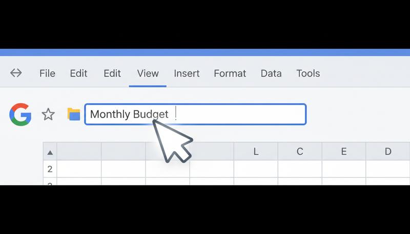
When you open a fresh spreadsheet, the top-left corner shows a placeholder: "Untitled spreadsheet." Time to give it a real name.
Click directly on those words. They become editable instantly. Type something meaningful—"Monthly Budget," "Book Tracking," "2024 Expenses," whatever—and press Enter. Your file now has an actual identity.
Now here's something that surprises almost everyone coming from Excel: Google Sheets saves automatically. There's no Ctrl+S habit to develop. Every change gets saved to the cloud within seconds. You'll catch a brief "Saving..." message at the top of the screen, which then shifts to "All changes saved in Drive." That's your signal that everything's secure.
This feels weird at first if you've spent years remembering to save before closing. But it's actually kind of liberating—no more panic about losing work because you forgot to hit save. The file lives in Google Drive from the moment you create it, and every single edit gets captured.
Remember: Autosave means you don't need to manually save in Google Sheets. But it does depend on internet connectivity. Lose your connection mid-session and Google Sheets will cache changes locally, syncing them back once you're online—but it's worth knowing that the safety net requires being plugged in.
A Guided Tour of the Interface
Your first look at Google Sheets can feel overwhelming. There's a lot of real estate, a lot of buttons, and a blank grid that stretches into infinity. Let's walk through it piece by piece—not just naming each part, but showing you when and why you'll actually reach for it.
The Menu Bar
Running across the very top: File, Edit, View, Insert, Format, Data, Tools, Extensions, Help. Click any of these and a dropdown menu appears with options inside. You don't need to memorize what's in each one—you'll pick up the layout naturally as you explore. For now, just know that if you're looking for a feature and can't find it in the toolbar, the menu bar is where you dig.
The Toolbar
Just below that sits a row of icons. This is where your quick-access formatting lives: bold, italic, font size, text color, background color, text alignment. If you've used Word, this will feel familiar. We'll dig into formatting later, but for now: whenever you want to change how something looks, the toolbar is your first stop.
The Formula Bar
Below the toolbar runs a long horizontal bar with an "fx" symbol on the left. This is the formula bar, and understanding it early will save you a lot of confusion later.
Here's what makes it special: the formula bar always shows you what's actually inside a cell, not just what the cell is displaying.
Try this right now. Click cell A1 and type 50, then press Enter. Click A1 again—the cell shows 50, and so does the formula bar. Easy. Now click cell B1, type =A1*2, and press Enter. The cell shows 100. But click B1 again and look at the formula bar—it shows =A1*2. The cell shows you the result; the formula bar shows you the instruction that produced it.
That distinction—result vs. instruction—is one of the most important things to understand about spreadsheets, and the formula bar is what makes it visible. When something is calculating unexpectedly, the formula bar is the first place you look.
The Name Box
To the left of the formula bar sits a small box displaying the address of your currently selected cell—"A1," "C4," whatever. This is the Name Box, and it does something surprisingly useful: click it, type any cell address, press Enter, and you jump there instantly. Working in a spreadsheet with thousands of rows? Type A1000 in the Name Box and hit Enter instead of scrolling forever. It's a small thing that earns its place quickly.
The Grid
The big white expanse in the middle is your actual spreadsheet. Columns are lettered (A, B, C...) across the top. Rows are numbered (1, 2, 3...) down the left side. Where a column and row intersect, you get a cell. Click any cell to select it, and you'll see both the column header and row number highlight—a little visual crosshair showing exactly where you are.
The Sheet Tabs
At the bottom of the window sit tabs labeled "Sheet1," "Sheet2," and so on. These sheet tabs let you navigate between multiple sheets within the same file. Think of your spreadsheet file as a notebook and each sheet as a page inside it. Right now you probably have just one tab—"Sheet1"—but you can have as many as you need.
Working with Sheet Tabs
Sheet tabs are more powerful than they look. Here's what you can do:
Rename a sheet: Double-click the tab name (or right-click and choose "Rename"), type something meaningful—"January," "Contacts," "Raw Data"—and press Enter. This sounds obvious, but you'd be surprised how many spreadsheets I've opened that still say Sheet1 through Sheet5—including ones I made myself before I learned better. Six months later, you'll thank yourself for naming them properly now, because "which Sheet3 has the real data?" is a genuinely annoying question to answer.
Add a new sheet: See the + button to the left of your existing tabs? Click it and a new sheet materializes.
Reorder sheets: Click and hold a tab, drag it to a new position, release. Useful when you have multiple sheets and want them in a logical order—say, January through December running left to right.
Color-code a sheet: Right-click a tab and choose "Change color." Give each sheet its own color, and suddenly navigating between them becomes faster. Red for "raw data," green for "summary," yellow for "in progress"—whatever system makes sense to you.
Delete a sheet: Right-click and choose "Delete." Google will ask you to confirm because deleted sheets are gone for good.
Warning: Sheet deletion is permanent. Deleting an entire sheet can be undone with Ctrl+Z just like deleting cell contents, as long as the deletion was the most recent action and no other changes have been made since. Double-check before you confirm.
Adjusting Column Width and Row Height
The default column width in Google Sheets is functional. But "functional" often means your text gets cut off and numbers show up as ### when they're too wide to fit. That ### display is just Google Sheets telling you "there's a number here but I don't have enough room to show it"—widen the column and it reappears.
To resize a single column manually: Hover your cursor over the border between two column headers—the line between column A and B in that gray row at the top. Your cursor changes to a double-headed arrow. Click and drag left or right to narrow or widen the column.
To auto-fit a column to its contents: Double-click that same column border and Google Sheets resizes it automatically to fit whatever's inside. No guessing, no manual dragging.
To resize multiple columns at once: Click the first column header, then Shift+click the last one you want to resize. Right-click any of the selected headers and choose "Resize columns." You can specify an exact pixel width or choose "Fit to data" to auto-size all of them at once.
Row height works identically—hover over the border between row numbers, drag to adjust, or double-click to auto-fit. Row height auto-fitting is especially useful when you've enabled text wrapping and some cells contain longer text that wraps across multiple lines.
Freezing Rows and Columns
Imagine you've built a spreadsheet with 50 rows of sales data. Row 1 contains your headers: Name, Date, Product, Amount. You scroll down to row 30 and suddenly can't remember which column is which because your headers disappeared off the top of the screen.
Freezing fixes this. A frozen row or column stays locked on screen no matter how far you scroll—it's pinned in place.
To freeze your header row:
- Click View in the menu bar
- Hover over Freeze
- Select 1 row
Now scroll down as far as you want. Row 1 stays put. The data moves underneath it, but your headers never leave the screen.
You can freeze multiple rows (useful if your headers take up two rows) and freeze columns too—same menu, same logic. Pick "1 column" to lock column A in place while you scroll right.
To unfreeze, go back to View → Freeze → No rows (or No columns).
Freezing feels like a small feature, but once you start working with real data, you'll use it constantly. It's one of those things that separates "technically works" from "actually pleasant to use."
Google Sheets vs. Microsoft Excel: Same Logic, Different Home
You've probably heard of Excel. Maybe you've used it, or maybe you've just seen it on other people's screens and assumed it's the "real" version of what we're doing. Let me clear that up.
Google Sheets and Excel are both spreadsheet applications, and they share identical fundamental logic—cells, rows, columns, formulas, functions, charts. Learn one well and you'll navigate the other without much struggle. The core concepts transfer completely.
The differences are practical rather than philosophical:
| Google Sheets | Microsoft Excel | |
|---|---|---|
| Cost | Free with a Google account | Paid (Microsoft 365 subscription) |
| Where it lives | In your browser (cloud-based) | Desktop app (with cloud sync available) |
| Autosave | Always on | Requires OneDrive or manual saving |
| Collaboration | Excellent—real-time, built-in | Good but feels bolted on |
| Formulas & functions | Comprehensive for most tasks | More extensive, especially for complex analysis |
| Spreadsheet size limit | Large (sufficient for nearly all everyday use) | Vastly larger (designed for enterprise-scale data) |
| Offline capability | Limited but functional | Strong offline operation |
On that size limit row: in practice, a typical household budget tracker might use 500 cells. A medium-sized business data export might use 50,000. You'd need to be doing serious enterprise-scale work—think large company databases or complex financial models—before either application's limits become relevant. For everything you'll build in this course, and most things you'll build for years afterward, Google Sheets has more than enough room.
For typical tasks—budgets, lists, trackers, basic data analysis—Google Sheets handles everything you'll need. Excel pulls ahead only when you're working with truly massive datasets, advanced statistical modeling, or need deep integration with Microsoft's business ecosystem.
Here's my practical take: start with Google Sheets. It's free, it's collaborative by default, it's accessible anywhere, and it'll teach you everything about how spreadsheets work. If you later encounter Excel at work, the transition will be smooth because the thinking behind it is identical.
Google even provides resources for switching from Excel to Sheets—which tells you something about how natural that jump tends to be.
You Now Have a Real Spreadsheet
Pause for a second and acknowledge what just happened. You created a spreadsheet that Google will keep safe indefinitely, that anyone in the world can view if you share a link, and that will automatically recalculate every number the moment you change one cell anywhere in it. That last part—the automatic updating—is what separates a spreadsheet from a static table, and it's exactly where we're headed next. The next section fills that grid with something real by walking you through the different types of data you can put in a cell—and why those differences matter more than you'd expect.
Only visible to you
Sign in to take notes.