How to Use Formulas in Google Sheets
You've now mastered the presentation side of spreadsheets — formatting that makes data readable, colors that guide the eye, layouts that communicate clearly. But here's the secret that separates a spreadsheet from a printed table: a spreadsheet can think. Formulas are what give it that power. They let you say: "Take the number in this cell, do something with it, and show me the result." And when the underlying numbers change, the result updates automatically. No calculator required. This is the moment everything changes — from a very pretty, static table into a living, calculating system.
Once that clicks, the rest of this course will feel obvious. Let's build that click.
What a Formula Actually Is
The Building Blocks
Before diving into what makes formulas so powerful, let's cover the basic arithmetic operators. These are just the symbols for the math you already know:
| Operator | Meaning | Example | Result |
|---|---|---|---|
+ |
Addition | =10+4 |
14 |
- |
Subtraction | =10-4 |
6 |
* |
Multiplication | =10*4 |
40 |
/ |
Division | =10/4 |
2.5 |
^ |
Exponentiation | =2^8 |
256 |
One thing that trips people up: multiplication uses * (not ×) and division uses / (not ÷). Your keyboard doesn't have those fancy math symbols, so spreadsheets use what's actually typeable. Same power, different notation.
Order of Operations: PEMDAS Still Rules
Google Sheets follows the same mathematical order of operations you learned in school — PEMDAS (Parentheses, Exponents, Multiplication, Division, Addition, Subtraction), or BODMAS if you learned it that way.
This matters more than you'd think. Compare:
=2+3*4→ 14 (not 20, because multiplication happens before addition)=(2+3)*4→ 20 (parentheses force the addition first)
When in doubt, use parentheses. They won't hurt anything, and they make your intention crystal clear — both to the spreadsheet and to future-you, reading this formula six months from now wondering what past-you was thinking.
The Real Power: Cell References
Here's where formulas go from neat trick to actually changing how you work.
Instead of typing actual numbers into your formula, you reference cells — and the formula uses whatever value is currently sitting in those cells. Change the cell, and your formula updates automatically.
Compare these:
Approach A: =150+75+30
Approach B: =B2+B3+B4
In Approach A, you've hard-coded the numbers. If rent jumps from 150 to 165, you have to edit the formula.
In Approach B, the formula reads whatever's currently in B2, B3, and B4. If B2 changes, your total updates instantly. You never touch the formula.
This is the fundamental shift that makes spreadsheets genuinely powerful. The W3Schools guide on references captures it well: references let formulas perform calculations on actual data wherever it lives, rather than numbers baked into the formula itself.
Think of a cell reference as a pointer, not a value. =B2 doesn't mean "use 150." It means "go look at B2 and use whatever you find there." That distinction is everything.
Tip: Get in the habit of putting your key numbers — tax rates, prices, conversion factors — in clearly labeled cells, then referencing those cells in your formulas. This makes your spreadsheet infinitely easier to update later.
Building Your First Formula: A Simple Budget
Let's make this concrete. Say you're tracking monthly expenses:
| Cell | Label | Value |
|---|---|---|
| A2 | Rent | 900 |
| A3 | Groceries | 280 |
| A4 | Transportation | 95 |
| A5 | Utilities | 65 |
You want a total in A6. Here's how to build that formula step by step:
- Click cell A6 — this is where your result appears.
- Type
=— this tells Sheets you're starting a formula. - Click cell A2 — Sheets inserts "A2" into your formula automatically. (Type it manually if you prefer — both work.)
- Type
+ - Click cell A3, type
+, click A4, type+, click A5 - Press Enter
Your formula is =A2+A3+A4+A5. Cell A6 now shows 1340.
Now change the value in A3 from 280 to 310. Watch A6 jump to 1370 instantly. You didn't touch the formula — it just recalculated. That's the spreadsheet doing what it was designed to do.
graph TD
    A2[A2: Rent = 900] --> Formula
    A3[A3: Groceries = 280] --> Formula
    A4[A4: Transportation = 95] --> Formula
    A5[A5: Utilities = 65] --> Formula
    Formula["Formula in A6: =A2+A3+A4+A5"] --> Result[A6 displays: 1340]
This is a tiny example, but the same principle scales to spreadsheets with thousands of rows and complex multi-sheet calculations. The logic stays identical.
The Formula Bar: Your Window Into What's Really There
That horizontal strip above your spreadsheet grid showing the cell address on the left and cell contents on the right — that's the formula bar, and it's doing something important.
When you click any cell, the formula bar shows what's actually inside that cell. If the cell contains a formula, you'll see the formula (like =A2+A3+A4+A5), while the cell itself displays the calculated result (1340). This two-layer reality — formula hiding behind the displayed number — is worth understanding clearly.
To read a formula: Click the cell and look at the formula bar.
To edit a formula: Click the formula bar directly and make changes, or double-click the cell to edit inline. Press Enter to confirm or Escape to bail without saving.
Here's something helpful: when you're editing a formula, Google Sheets color-codes the cell references and highlights the matching cells on the spreadsheet in the same colors. If A2 appears in blue in the formula, cell A2 gets a blue border. This makes it easy to verify you're referencing the right cells. AbleBits specifically highlights this feature — it's one of those small details that actually makes debugging much less painful.
Relative References: The Magic of Copying Formulas
Here's a common scenario: you've built that budget formula for January. Now you want the same calculation for February through December — in separate columns. Do you rebuild the formula eleven more times?
No. You copy it. And this is where relative references become surprisingly useful.
By default, every cell reference in a formula is relative. "Relative" means: "I'm not pointing to one specific fixed cell — I'm pointing to a cell that's X rows away and Y columns away from where I am."
In practice, here's what happens. Your formula in B6 is =B2+B3+B4+B5. You copy it to C6. Sheets doesn't paste the same formula there. It pastes =C2+C3+C4+C5. Because the formula means "add the four cells directly above me" — and in column C, that's C2 through C5.
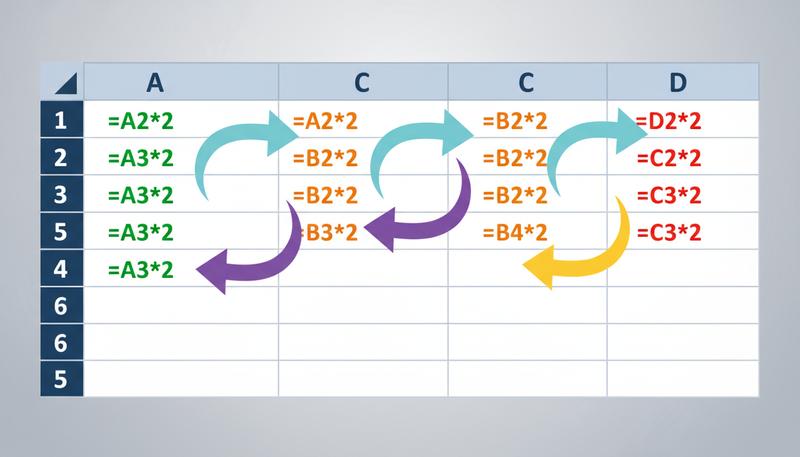
This is enormously useful. Write a formula once, copy it across 12 columns, and each column's formula automatically uses its own column's data. The W3Schools reference guide shows this with a practical example — relative references give the fill function "freedom to continue the order without restrictions."
A relative reference says "use the cell over there relative to me," not "use the cell with this exact address." The difference is everything.
Absolute References: When You Need Something to Stay Put
Relative references are wonderful — until you need something to stay fixed.
Imagine you have a tax rate in cell D1 (say, 8%), and you're calculating tax on a series of prices in column B. Your formula in C2 is =B2*D1.
Copy that down to C3, C4, C5, and relative references shift it: D1 becomes D2, D3, D4. But there's no tax rate in those cells. You only have it in D1. Your formula silently breaks, pulling wrong numbers or zeros.
You need to say: "Keep pointing at D1 — don't adjust this reference when I copy the formula." That's an absolute reference, created with the dollar sign ($).
Change your formula to =B2*$D$1. Now:
B2is relative — it shifts as you copy down (B3, B4, etc.)$D$1is absolute — it always points to D1, no matter where you copy
The $ before the column locks the column. The $ before the row locks the row. Use both ($D$1) and the entire reference is frozen.
Warning: Forgetting absolute references when you need them is one of the most common formula bugs. If you copy a formula and get weird results, check whether a reference should have been absolute.
Quick shortcut: F4 is not the standard shortcut for cycling reference types in Google Sheets. While F4 works this way in Microsoft Excel, Google Sheets does not have a standard F4 shortcut for cycling through absolute/relative references. Users must manually edit the $ symbols or use other methods.: D1 → $D$1 → D$1 → $D1 → back to D1. Saves a lot of typing.
Mixed References: Locking Just What You Need
Once relative and absolute references make sense, mixed references are straightforward: they lock either the row or the column, not both.
$D1— column is locked (D stays D), row is relative (1 shifts as you copy)D$1— row is locked (1 stays 1), column is relative (D shifts as you copy)
When do you use this? The classic case is a multiplication table or pricing grid. Say you have sizes across the top (row 1) and materials down the left (column A), and you want every cell to multiply its row's size by its column's material cost.
The formula in B2 would be =$A2*B$1:
$A2— always look in column A for the material, but move down the rowsB$1— always look in row 1 for the size, but move across the columns
Copy that formula anywhere in the grid and it stays correct. This is advanced territory, and you might not need it for a while — but knowing it exists will save you from a future puzzle moment.
The Fill Handle: Your Best Friend for Copying
Now that you understand relative and absolute references, let's talk about the fastest way to copy formulas: the fill handle.
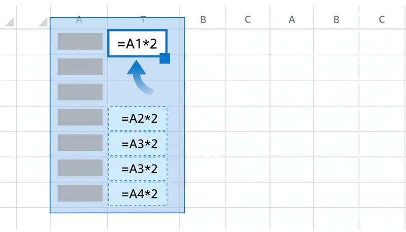
Look at the bottom-right corner of any selected cell. You'll see a tiny blue square. That's the fill handle. Click and drag it in any direction, and Google Sheets copies your formula into each cell you drag through — adjusting the relative references automatically.
To fill down a column: Type your formula in the first cell, then grab the fill handle and drag downward through the cells you want to fill.
To fill across a row: Same idea, but drag sideways.
The fast double-click trick: If your adjacent column already has data, just double-click the fill handle instead of dragging. Sheets will automatically fill down as many rows as your neighboring column has data. This is a huge time-saver with large datasets.
Common Formula Errors (And What They Mean)
Errors happen. They're not a catastrophic sign — they're the spreadsheet's way of saying "I tried to run your formula but hit a problem." Here are the main ones:
#DIV/0! — You're dividing by zero (or by an empty cell, which counts as zero). Usually this means a referenced cell is blank when it shouldn't be, or you've set up a ratio before entering all your data.
#VALUE! — The formula got the wrong type of data. For example, you tried to multiply a number by text. This often happens when a cell looks like it has a number but actually contains text (a common problem when importing data).
#REF! — A cell reference is broken — usually because you deleted a row or column that the formula was pointing to. The cell it referenced literally doesn't exist anymore.
#NAME? — Google Sheets doesn't recognize something in your formula. Usually you've misspelled a function name or forgot the = at the start.
###### — Not technically an error, just a display issue. The column is too narrow to show the number. Widen it and it displays normally.
Tip: When you see an error, click the cell and look at the formula bar. Read the formula carefully. Then ask: "Is every reference pointing to a cell that exists? Does every cell have the data type I expect?" Those two questions solve most formula errors.
Putting It Together: The Dynamic Budget in Action
Let's step back and recognize what you've just learned, because it's more significant than it might feel.
You can create formulas that calculate results from cell values. Those formulas update automatically when the values change. You can copy formulas efficiently using the fill handle, and relative references mean the copied formulas adjust intelligently. Absolute references let you lock in a constant — like a tax rate or discount percentage — that every formula can reference. And when things go wrong, error messages give you a starting point for investigation.
This is the foundation everything else in this course builds on. Functions (coming next) are just formulas with pre-built capabilities — they use the same =, the same cell references, the same fill handle, the same error system. Charts pull from the same cells your formulas calculate into. Cross-sheet lookups use the same reference logic, just extended to other tabs.
You've essentially learned the grammar of spreadsheets. Everything from here is vocabulary.
One final thought: the real payoff of formulas isn't any single calculation. It's the ability to change your input data and watch all your conclusions update simultaneously. A budget spreadsheet built with proper cell references doesn't just tell you your current total — it lets you ask "what if rent goes up 10%?" and see the ripple effect across every calculation in seconds. That's not accounting software magic. That's just a formula reading from a cell.
And you know how to do that now.
Only visible to you
Sign in to take notes.