Building a Real-World Spreadsheet from Scratch
Putting It All Together: Building a Real-World Spreadsheet from Scratch
By now, you've picked up every major tool Google Sheets has to offer: data entry, formatting, formulas, functions, lookups, sorting, filtering, charts. You've learned how to share your work and keep it safe. But here's the thing about learning tools in isolation — they're just tools until you see how they fit together in the real world. That's what this final section is really about.
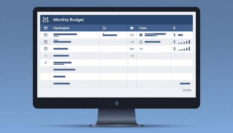
You're going to build a complete, functional personal monthly budget tracker. From a blank grid to a finished, formatted, chart-equipped spreadsheet you could actually use to manage your money. Every step draws on something you've learned: data types, formulas, SUMIF, IF, formatting, charts, cross-sheet references, VLOOKUP, conditional formatting. Nothing gets wasted. By the end, you won't just have a budget tracker. You'll have proof that you understand how spreadsheets actually work.
Before You Start: Why Structure Matters
Here's something most people get wrong their first time: mixing structure and data. They'll dump raw transactions in one column and calculations in another, and suddenly updating a number breaks three other things.
Don't do that.
Your raw transactions belong in one place. Calculations belong somewhere else. Don't sum things in the same column where your data lives. Future-you will be genuinely grateful for this small act of kindness.
Step 1: Create a New Spreadsheet
Head to Google Sheets and create a new spreadsheet. Name it something meaningful like Monthly Budget — October 2024 — click the title at the top left and type it in.
You'll notice the default sheet tab at the bottom says "Sheet1". Right-click it and rename it Transactions. This is where the raw data lives.
Step 2: Set Up Your Column Headers
Type your column headers in Row 1:
- A1: Date
- B1: Description
- C1: Category
- D1: Type
- E1: Amount
Now select the entire first row. Make it bold (Ctrl+B or Cmd+B), then give it a background color — something calm, like medium blue or slate gray. This header row should visually announce itself as the start of your data.
Your spreadsheet has a skeleton now. It's empty, but it has structure. And structure is everything.
Step 3: Enter Some Real Data
Time to fill the skeleton. Enter these sample transactions starting in Row 2. (They're realistic but fictional — feel free to swap in numbers from your own life if you want to make this genuinely useful right away.)
| Date | Description | Category | Type | Amount |
|---|---|---|---|---|
| 10/1 | Paycheck | Income | Income | 3500 |
| 10/3 | Apartment rent | Housing | Expense | 1200 |
| 10/5 | Groceries | Food | Expense | 180 |
| 10/7 | Netflix | Entertainment | Expense | 15 |
| 10/8 | Gas | Transport | Expense | 60 |
| 10/10 | Freelance project | Income | Income | 800 |
| 10/12 | Restaurant dinner | Food | Expense | 75 |
| 10/15 | Electricity bill | Housing | Expense | 95 |
| 10/18 | Gym membership | Health | Expense | 45 |
| 10/20 | Grocery run | Food | Expense | 130 |
| 10/22 | Spotify | Entertainment | Expense | 10 |
| 10/25 | Bus pass | Transport | Expense | 90 |
| 10/28 | Pharmacy | Health | Expense | 35 |
Just enter all 13 rows. Don't format anything yet — the raw data comes first.
Once it's in, look at what you've built. Clean rows, one transaction per line, consistent categories, no merged cells, no decorative chaos. This is exactly how Google Sheets expects data to be organized when you want to sort it, filter it, chart it, or calculate with it. This structure is what makes everything else possible.
Step 4: Write Formulas to Total Each Category
Now we find out what this data actually means. We need to know how much was spent in each category. You could add up the numbers by hand, but that defeats the entire purpose.
Below your last data row (Row 15), leave a blank line for breathing room. Starting in Row 17, add your summary labels:
- C17: Housing
- C18: Food
- C19: Transport
- C20: Entertainment
- C21: Health
- C22: Total Expenses
- C23: Total Income
- C24: Net Income
In cell D17, you'll write your first SUMIF formula. (SUMIF is like a smarter SUM — it only adds up values that meet a condition, which is exactly what you need to total by category.)
=SUMIF(C2:C14,"Housing",E2:E14)
Translation: Look through column C. Wherever you find "Housing", add up the corresponding value in column E.
Do the same for the other categories:
- D18:
=SUMIF(C2:C14,"Food",E2:E14) - D19:
=SUMIF(C2:C14,"Transport",E2:E14) - D20:
=SUMIF(C2:C14,"Entertainment",E2:E14) - D21:
=SUMIF(C2:C14,"Health",E2:E14)
For total expenses, you'll sum everything marked as an "Expense" in the Type column:
- D22:
=SUMIF(D2:D14,"Expense",E2:E14)
And total income:
- D23:
=SUMIF(D2:D14,"Income",E2:E14)
Finally, the simplest formula in the whole sheet — your bottom line:
- D24:
=D23-D22
The magic here is that each cell reference points to live data. Change a transaction amount and every total updates instantly. That's why structure matters — the calculations sit separate from the raw data, so they can just keep working.
Remember: SUMIF takes three arguments: the range to check, the condition you're looking for, and the range to sum. Get those three in the right order and you can filter-sum almost anything.
Step 5: Use IF to Flag When You're Over Budget
A budget that just shows totals is useful. One that tells you when you've gone over budget? That's actually actionable.
Add two new columns to your summary section. In E17, start entering some reasonable monthly budgets for each category:
- E17: 1300 (Housing)
- E18: 350 (Food)
- E19: 100 (Transport)
- E20: 30 (Entertainment)
- E21: 50 (Health)
Add a header in E16 that says "Budget" and another in F16 that says "Status".
Now in F17, write:
=IF(D17>E17,"⚠ OVER BUDGET","✓ OK")
Copy this down to F18:F21.
This is the IF function doing what it was designed for: making a decision based on a condition. If the actual spending (D17) exceeds the budget (E17), it flags it with a warning. Otherwise, it gives you a green light. The spreadsheet re-evaluates this automatically every time you update a transaction.
With the sample data, Entertainment ($25) and Housing ($1,295) should be fine, but Food ($385) and Transport ($150) will flash warnings. Your spreadsheet just told you something useful.
Step 6: Format Your Numbers as Currency
Your Amount column currently displays raw numbers like 3500 and 180. Those should look like money.
Select all the cells in column E that contain amounts (E2:E14), plus your summary totals (D17:D24). Then:
- Go to Format → Number
- Choose Currency
Everything now displays as proper currency: $3,500.00, $180.00. Consistent and professional.
Here's a useful thing to know: Google Sheets' number formatting is just a costume. The underlying value is still 3500 — the format is just how it looks on screen. Your formulas keep working correctly because they're looking at the actual numbers, not the dressed-up versions.
While you're formatting, make the labels in C22:C24 bold. Make D24 (your Net Income) slightly larger. Visual hierarchy helps — your eye should land on that bottom number first.
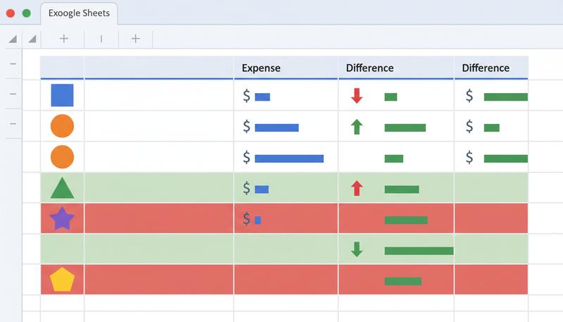
Step 7: Add Conditional Formatting to Highlight Problems
The IF flag in column F tells you when something's wrong. But sometimes you want the whole row to jump out at you. That's what conditional formatting is for.
Select your summary table: C17:F21. Then:
- Go to Format → Conditional formatting
- Under "Format cells if," choose Custom formula is
- Enter:
=$D17>$E17 - Pick a red background
- Click Done
The dollar signs lock the column letters but let the row numbers shift — so the rule applies correctly to each row. Any category where spending exceeds budget now glows red.
Add another rule: same range, but this time use =$D17<=$E17 and pick a green background. Now your summary table becomes a traffic light — instant visual communication of what's on track and what isn't.
Step 8: Create a Pie Chart
Your numbers are accurate, but a visual can communicate the same story in two seconds. Let's add a pie chart.
Select your category names and their totals: C17:D21 (Housing through Health). Then:
- Click Insert → Chart
- Google Sheets will likely default to a bar chart. In the Chart Editor panel on the right, change Chart type to Pie chart
- Make sure the Data range is set to
C17:D21
Give your chart a title: October Expenses by Category.
Move the chart to sit to the right of your summary table. Now you have both the numbers and the visual. Housing will dominate the pie (as it should), and Entertainment will be a tiny sliver. Anyone looking at this chart understands your spending instantly.
The beautiful part about Google Sheets charts is that they're live. Add a new transaction next month and the pie chart updates automatically.
Step 9: Create a Summary Sheet with Cross-Sheet References
Now you're going to build the next layer up: a high-level view that pulls from the detailed data.
Right-click the + button at the bottom to add a new sheet. Rename it Monthly Summary.
Set up these column headers:
- A1: Month
- B1: Total Income
- C1: Total Expenses
- D1: Net Income
In A2, type: October
Now for the clever part. In B2, instead of manually retyping the income total, pull it directly from the Transactions sheet:
=Transactions!D23
That exclamation point syntax says: "Go to the Transactions sheet and grab cell D23." Whatever lives there — even if it changes — appears here.
Fill in the rest the same way:
- C2:
=Transactions!D22 - D2:
=Transactions!D24
Format B2:D2 as currency. Now your Monthly Summary sheet is a clean, high-level snapshot that stays in sync with your detailed data automatically. When you have large datasets spread across multiple sheets, cross-sheet references like this are genuinely powerful.
Step 10: Use VLOOKUP to Pull Category Descriptions
This step gets a bit advanced, but it shows something important: VLOOKUP isn't just for looking things up in existing data — it lets you maintain a separate reference table and pull from it on demand.
Go back to the Transactions sheet. Scroll down past your summary section to around Row 28. Create a small reference table:
| Category Code | Full Description |
|---|---|
| Housing | Rent, utilities, and home maintenance |
| Food | Groceries, dining out, and delivery |
| Transport | Gas, transit, and rideshare |
| Entertainment | Streaming, events, and hobbies |
| Health | Gym, pharmacy, and medical |
Type this in H1:I6 (H1 as "Category Code", I1 as "Full Description").
Now go back to your Monthly Summary sheet. Add a new column E1 labeled "Category" and F1 labeled "Description". In E2, type Housing. In F2, write:
=VLOOKUP(E2,Transactions!H2:I6,2,FALSE)
This says: Take the value in E2, look it up in the first column of that range on the Transactions sheet, and return the value from the second column of whichever row matches.
Result: "Rent, utilities, and home maintenance" appears in F2.
You've just used VLOOKUP as a documentation tool — something most people never think to do with it, but it's genuinely useful.
Warning: VLOOKUP is case-insensitive in Google Sheets, but it will care about trailing spaces. If your reference table says "Housing" and the lookup value says "Housing " (with a space at the end), it fails silently. If you see #N/A, suspect whitespace before you suspect the formula.
Step 11: Freeze Headers and Add Alternating Row Colors
Two quick polish touches that make a huge difference in real-world usability.
First, freeze the header row. Go back to the Transactions sheet. Click on Row 1, then go to View → Freeze → 1 row. Now when you scroll down through months of transactions, your column headers stay locked at the top. Seems minor until you have 200 rows of data.
Second, add alternating row colors. Select your data range A1:E14. Go to Format → Alternating colors and pick a palette you like. Click Apply.
Alternating row colors (sometimes called "zebra striping") make it dramatically easier to read across a wide row without losing your place. Pure readability, accomplished in about ten seconds.
Step 12: Share and Annotate
Your spreadsheet is done. Now share it.
Click Share in the top right. In the dialog:
- Type an email address
- Change permission from Editor to Viewer — this is read-only access. They see everything but can't change anything
- Uncheck "Notify people" if you don't want to send an email
- Click Share
Now add a comment to clarify something important. Go to cell D24 (Net Income) on the Transactions sheet. Right-click and choose Insert comment. Type something like: "This is the bottom line — it should be positive. If it's negative, we have a problem."
Click Comment. A small orange triangle appears in the cell corner. Anyone with access can hover over it to read your note.
Google Sheets' collaboration happens in real time — if both people are in the document simultaneously with Edit access, you'll see each other's cursors moving. For a budget tracker shared with a partner, this is genuinely useful.
What You Actually Built
Let's inventory what's sitting in this single spreadsheet:
- ✅ Clean, structured data entry
- ✅ SUMIF formulas aggregating by category
- ✅ IF function flagging over-budget categories
- ✅ Currency number formatting
- ✅ Conditional formatting with red/green alerts
- ✅ A pie chart showing expense breakdown
- ✅ A second sheet with cross-sheet references
- ✅ VLOOKUP pulling from a reference table
- ✅ Frozen headers and alternating row colors
- ✅ View-only sharing and comments
That's the entire course, assembled into one real thing that solves an actual problem. You didn't just learn about spreadsheets. You built something that works.
Where to Go From Here
You've covered the fundamentals, but honest truth: spreadsheets go as deep as you want them to. Here are the next natural steps:
Data validation — Limit what can be entered in a cell before errors happen. Make the Category column a dropdown so it only accepts your defined categories. No more typos turning "Food" into "Foood" and breaking your SUMIF. Look for Data → Data validation.
Pivot tables — The single most powerful feature for summarizing large datasets. A pivot table can answer "how much did I spend on food in each month of the year?" in about four clicks. Google has a solid guide to pivot tables worth bookmarking.
Advanced functions — Once IF and VLOOKUP are comfortable, the next tier includes COUNTIF (count rows meeting a condition), AVERAGEIF (average by category), INDEX/MATCH (more flexible than VLOOKUP), and QUERY (filter and sort using something resembling English). Each one extends the same logic you already understand.
Google Sheets add-ons — The marketplace has hundreds of add-ons for everything from mail merge to advanced charting to database connectivity. Once you're fluent in the basics, add-ons let you solve specialized problems without building from scratch.
Remember: The goal was never to memorize every function Google Sheets has. It was to understand how spreadsheets think — so you can reason your way through new problems yourself. Every formula you'll ever write is just a combination of the same ideas: reference a cell, apply some logic, return a result. You already know that. The rest is just vocabulary.
Final Thought
There's a moment when learning something new switches from feeling like disconnected pieces to feeling like one coherent system. Maybe it happened when a VLOOKUP clicked, or when conditional formatting did exactly what you wanted, or when you realized a pie chart was just a visual translation of a formula you'd already written.
If that moment happened somewhere in this course — that's what it was all about.
Spreadsheets aren't magic, and they're not just for people who "do numbers." They're a way of thinking: structured, logical, curious about outcomes. You have that now.
Go build something.
Only visible to you
Sign in to take notes.