Understanding Spreadsheet Rows Columns Cells and Sheets
You now understand what spreadsheets do — they hold information and let you update it over time. But before you open Google Sheets and start building, you need to understand what a spreadsheet actually looks like and how it's organized. Let's take a closer look at the anatomy of a spreadsheet: the rows, columns, cells, and sheets that make up the structure you'll be working with.
Here's something that separates confident spreadsheet users from people who constantly feel lost: they have a clear mental map of how these pieces fit together. Once you have that map, everything else — formulas, formatting, sharing — clicks into place naturally. It's like learning the names of chess pieces before learning to play; you could stumble around without the vocabulary, but you'd constantly be confused about what you're looking at. Get the language down first, and the rest of the game starts to make sense.
So let's take a tour of the spreadsheet, piece by piece.
Rows and Columns: The Foundation
A spreadsheet is fundamentally a grid. That grid has two directions: rows and columns.
Rows run horizontally across the page, and they're numbered: 1, 2, 3, 4... Google Sheets starts every new spreadsheet with 26 rows by default (though the exact default visible rows may vary; it generates additional rows as users scroll down) — more than enough for most everyday tasks. If you need more, you can add them; the software can handle millions of cells total, so space is rarely a real constraint.
Columns run vertically down the page, and they're lettered: A, B, C, D... all the way to Z, then AA, AB, AC, and beyond (the vast majority of real-world spreadsheets never venture past column Z, but Google Sheets has them ready if you do).
The reason columns use letters and rows use numbers is purely practical: it gives every cell a unique, unambiguous address using one letter and one number, rather than two numbers that might be easy to confuse. More on that in a moment.
Think of columns as categories or attributes. In an expense tracker, column A might be "Date," column B might be "Description," column C might be "Amount." Each column holds the same kind of information for every row.
graph LR
    A[Column A\nDate] --> R1[Row 1: Jan 5]
    A --> R2[Row 2: Jan 12]
    A --> R3[Row 3: Jan 20]
    B[Column B\nDescription] --> R4[Row 1: Groceries]
    B --> R5[Row 2: Gas]
    B --> R6[Row 3: Netflix]
    C[Column C\nAmount] --> R7[Row 1: $84.50]
    C --> R8[Row 2: $45.00]
    C --> R9[Row 3: $15.99]
Cells: Where the Magic Lives
Here's the most important concept in this whole section: a cell is the intersection of a row and a column. Every single piece of data you'll ever enter in a spreadsheet lives inside a cell.
That's it. One cell, one piece of information.
Cells are the fundamental unit of a spreadsheet — like atoms in chemistry, or pixels on your screen. Everything else is built from them. You can think of the grid as just a very organized collection of cells, each one patiently waiting to hold something.
A cell can hold:
- A number (like
42or3.14) - Text (like
"Revenue"or"Maria Johnson") - A date (like
January 5, 2024) - A formula (like
=A1+B1, which calculates a value from other cells) - Nothing at all (blank cells are perfectly fine and very common)
Remember: One cell, one piece of information. This sounds obvious, but it's the rule that beginners most often break — stuffing "First and Last Name" into a single cell instead of using two separate cells. Keeping data atomic (one piece per cell) makes everything else — sorting, filtering, formulas — work much more smoothly.
Cell Addresses: The Spreadsheet's Street Map
Since every cell is the intersection of a column and a row, every cell has a unique address made of the column letter followed by the row number.
- The cell in column A, row 1 → A1
- The cell in column B, row 3 → B3
- The cell in column Z, row 100 → Z100
This naming system is called A1 notation, and it was first introduced in the early spreadsheet program LANPAR back in 1969. It's been the standard ever since, across virtually every spreadsheet program on the planet.
Reading a cell address is simple: column first, row second. So B5 means "column B, row 5" — like reading a map coordinate where you go across before you go up. (If you've ever played the game Battleship, it's the exact same idea.)
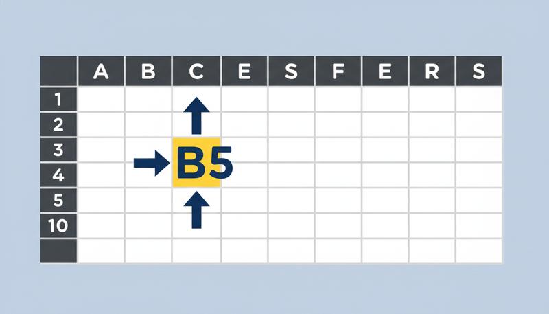
You'll see cell addresses constantly as you work — in formulas, in error messages, in your own notes about where you put things. Getting comfortable reading them is like learning to read street addresses: it takes about five minutes, and then it's second nature.
Ranges: Selecting Groups of Cells
A range is simply a group of cells treated as a unit. Instead of referring to cells one at a time, you can refer to a whole block of them with a single notation.
The format is: starting cell : ending cell, using a colon between them.
A1:A10— all cells in column A, rows 1 through 10 (a vertical stripe)A1:C1— all cells in row 1, columns A through C (a horizontal stripe)A1:C5— a rectangular block: columns A through C, rows 1 through 5 (fifteen cells total)
Ranges are the shorthand that makes working with lots of cells feel manageable rather than tedious. You'll use them all the time. When you want to sum a column of numbers, you'll tell the spreadsheet to sum the range B2:B20. When you want to format a header row, you'll select the range A1:F1.
Tip: To select a range with your mouse, click the first cell, hold Shift, and click the last cell. The whole block will highlight in blue. You can also click and drag. Either way, the range address will appear in the Name Box as you select it.
Worksheets and Workbooks: The File Cabinet Analogy
So far we've been talking about a single grid. But spreadsheet files can contain multiple grids, and understanding the relationship between them is important.
Here's the analogy: think of a workbook (the entire file) as a three-ring binder. Inside that binder, you have multiple worksheets (also called sheets or tabs) — these are the individual pages inside the binder.
In Google Sheets, you'll see your worksheets as tabs at the bottom of the screen. By default, a new file starts with one sheet called "Sheet1." You can:
- Add more sheets (click the
+button next to the existing tabs) - Rename them (double-click the tab name)
- Reorder them (drag the tabs around)
- Color-code them (right-click a tab for options)
Why use multiple sheets? Here's a common real-world pattern: imagine you're tracking your household budget. You might have:
- A sheet called January with all your January expenses
- A sheet called February with February expenses
- A sheet called Summary that pulls totals from both monthly sheets into one overview
Same workbook (one file), three organized worksheets. Much cleaner than cramming everything onto a single enormous grid.
When you reference a cell from a different sheet, the address gets the sheet name added: Sheet1!A1 means "cell A1 on the sheet named Sheet1." The exclamation mark is the separator. We'll cover cross-sheet references in detail when we get to looking things up — for now, just know that the notation exists.
graph TD
    WB[Workbook\n📁 Budget 2024.xlsx]
    WB --> S1[Sheet: January]
    WB --> S2[Sheet: February]
    WB --> S3[Sheet: Summary]
    S1 --> C1[Cells A1:D50]
    S2 --> C2[Cells A1:D48]
    S3 --> C3[Pulls from\nJanuary + February]
The Interface: A Quick Map
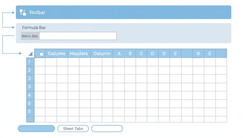
Now let's zoom out and look at the Google Sheets interface as a whole. When you open a spreadsheet, you're looking at several distinct zones, each with a specific job.
The Toolbar runs across the top of the screen, below the menu bar. It's a row of buttons for formatting: making text bold, changing font size, adding borders, aligning content, and more. Think of it as your formatting palette. You'll use it often once your data is in place.
The Formula Bar sits just above the column headers (A, B, C...). When you click on a cell, the formula bar shows you exactly what's inside that cell — not just what it displays. This distinction matters: a cell might display $1,250.00 but the formula bar reveals it actually contains =B3*1.1. The formula bar is the truth-teller.
The Name Box sits to the left of the formula bar. It shows the address of the currently selected cell — click on D7 and it displays D7, click on A1 and it shows A1. But it does more than display: you can type into it. Click the Name Box, type Z50, press Enter, and you'll instantly jump to cell Z50, no matter where you are in the sheet. It's a teleporter, and it's the correct Google Sheets way to navigate directly to a specific cell. Use it whenever scrolling feels like more work than it's worth.
The Grid takes up most of the screen. This is your canvas — the actual spreadsheet where you enter and view data.
The Sheet Tabs run along the very bottom. Each tab is one worksheet within the workbook. You can have as many as you like.
Navigating the Grid: Keyboard Shortcuts Worth Knowing
Here's something experienced spreadsheet users know: the mouse is slow. Once you're comfortable with the keyboard, you'll zip around a spreadsheet at twice the speed.
These are the essential navigation shortcuts for Google Sheets:
| Action | Shortcut (Windows) | Shortcut (Mac) |
|---|---|---|
| Move one cell in any direction | Arrow keys | Arrow keys |
| Move to next cell (data entry) | Tab (right) / Enter (down) | Tab / Enter |
| Jump to the edge of a data region | Ctrl + Arrow key | Cmd + Arrow key |
| Jump to cell A1 | Ctrl + Home | Cmd + Fn + ← |
| Jump to last cell with data | Ctrl + End | Cmd + Fn + → |
| Select a range | Shift + Arrow keys | Shift + Arrow keys |
| Select to edge of data | Ctrl + Shift + Arrow | Cmd + Shift + Arrow |
| Go to a specific cell | Type address in the Name Box | Type address in the Name Box |
The Ctrl + Arrow shortcut (or Cmd + Arrow on Mac) deserves special attention. If you're in the middle of a column of data and press Ctrl + Down, you'll jump to the last filled cell before a gap. It's like a turbo scroll. Press it when you're in an empty cell and you'll fly all the way to the edge of the sheet's data region.
Tip: Press Ctrl + End (Cmd + Fn + → on Mac) to jump to the last cell that contains data in your sheet. This is a handy way to find out how far your spreadsheet actually extends. Keep in mind that Google Sheets starts with 1,000 rows by default, so if you press Ctrl + End in a brand-new sheet and land somewhere around Z1000, that just means the sheet is empty — not that you have thousands of rows of data. If you find yourself with hundreds of empty rows you don't need, you can select and delete them to keep things tidy and help the file run a touch faster.
Putting It Together: A Mental Model
Let's make sure the whole picture is clear before we move on.
A workbook is a file. Inside it live one or more worksheets (the tabs). Each worksheet is a grid of rows (horizontal, numbered) and columns (vertical, lettered). Every cell is the intersection of one row and one column, and it holds exactly one piece of information. Every cell has a unique address (like B4). Groups of cells form ranges (like B4:D12).
That's the entire vocabulary. Six words: workbook, worksheet, row, column, cell, range. Master these, and every tutorial, help article, and formula reference you encounter will make sense — because they all use this same language.
In the next section, we'll actually open Google Sheets and create your first spreadsheet. Now that you have the map, it's time to start exploring the territory.
Only visible to you
Sign in to take notes.