How to Use Google Sheets Functions and Formulas
You've just mastered the foundation: formulas that calculate, copy intelligently, and update in real time. Now it's time to level up. While you can add 200 numbers by typing =A1+A2+A3+...+A200, Google Sheets offers something far better: functions — pre-built operations designed to handle exactly these kinds of repetitive or complex tasks. If formulas are the grammar of spreadsheets, functions are the vocabulary that lets you say more with less.
Functions are named operations that take some inputs (called arguments), process them, and return a single result to your cell. Think of them like appliances in your kitchen: you could whisk eggs by hand, but a stand mixer does it faster and better. The handful of functions we'll cover here — SUM, AVERAGE, COUNT, MIN, MAX, and IF — will handle something like 80% of what most people ever actually need a spreadsheet to do. Master these, and you'll already be more capable than the average person who claims to "use Excel." The good news? They're built on exactly the same logic as the formulas you just learned — same = sign, same cell references, same error system.
Entering Functions: Let Google Sheets Help You Type
Before we dive into specific functions, here's a technique that'll save you typing and prevent typos: AutoComplete.
When you type = in a cell and start typing a function name, Google Sheets immediately shows you a dropdown of matching functions. As you type more letters, the list narrows. When you see the one you want, you can press Tab to accept it — the opening parenthesis is added automatically.
Even better: once you've typed the function name and the opening parenthesis, Google Sheets shows you a little tooltip explaining what the function does and what arguments it expects. You'll see something like:
SUM(value1, [value2, ...])
That tooltip is your in-line documentation. It's showing you that SUM needs at least one argument (value1), and can optionally take more (the [value2, ...] in brackets).
Tip: Never dismiss that tooltip by clicking elsewhere. It disappears when you close the parenthesis or press Enter. While it's visible, it's actively telling you what the current argument expects — a genuinely useful feature that beginners often ignore.
As the Ablebits guide notes, Google Sheets will suggest all matching functions starting with whatever letters you've typed. This is especially helpful when you half-remember a function name — type the first few letters and let the autocomplete do the rest.
SUM: The Most-Used Function in the World
If there's a Mount Everest of spreadsheet functions, it's SUM. This is the one that adds up numbers in a range, and it's almost certainly the first function every new spreadsheet user learns.
Syntax: =SUM(value1, [value2, ...])
The argument can be:
- A single cell:
=SUM(B2)(not very useful, but valid) - A list of cells:
=SUM(B2, B5, B9)(adds those three specific cells) - A range:
=SUM(B2:B10)(adds every cell from B2 through B10) - Multiple ranges:
=SUM(B2:B10, D2:D10)(adds two separate ranges)
In practice, you'll use the range version almost exclusively. Here's why it's so much better than adding cells manually: imagine you have a column of 50 sales figures. With manual addition, you'd need to type all 50 cell references. With SUM, you just type =SUM(B2:B51). Done.
And here's the magic: if you change any value in that range, the sum updates automatically. If you accidentally type a negative number, as W3Schools illustrates with their Pokémon stats example, SUM will correctly subtract it — it adds up all values, positive or negative, faithfully.
A practical example: You're tracking your monthly grocery spending across four weeks:
| Week | Amount |
|---|---|
| Week 1 | $127.50 |
| Week 2 | $89.30 |
| Week 3 | $143.20 |
| Week 4 | $104.80 |
| Total | =SUM(B2:B5) |
Your formula in B6 would be =SUM(B2:B5) and it would return $464.80. Add another week? Adjust the range to B2:B6 and it'll include it. The spreadsheet updates; you don't have to.
AVERAGE: Finding the Middle Ground
AVERAGE does exactly what you'd expect: it calculates the arithmetic mean of a range of numbers. Add them all up, divide by the count. The function handles both steps so you don't have to.
Syntax: =AVERAGE(value1, [value2, ...])
=AVERAGE(B2:B5)
Using the grocery example above, =AVERAGE(B2:B5) would return $116.20 — your average weekly grocery spend.
This is where functions start revealing their true power. Without AVERAGE, you'd need: =(B2+B3+B4+B5)/4. That works fine with four numbers, but what if you had 52 weeks of data? You'd need to write =(B2+B3+...+B53)/52. With AVERAGE, it's just =AVERAGE(B2:B53) regardless of how many numbers are in the range.
One thing to know: AVERAGE ignores empty cells but includes cells with a zero value. This matters. If you have a range with 10 cells but only 7 have values, AVERAGE divides the total by 7, not 10. This is usually the behavior you want — it doesn't penalize you for having blank rows — but it's worth knowing.
Remember: AVERAGE ignores blank cells but counts zeros. If a week had $0 in spending (miraculous), it counts. If you just left the cell blank (because you forgot to enter the data), it doesn't count. These are very different situations, so make sure your blanks are intentional.
COUNT and COUNTA: When You Need to Know How Many
Sometimes you don't want to add numbers up — you want to count how many there are. Google Sheets gives you two functions for this, and knowing the difference is important.
COUNT counts cells that contain numbers.
Syntax: =COUNT(value1, [value2, ...])
=COUNT(B2:B10)
If B2:B10 has 7 cells with numbers and 2 empty cells, COUNT returns 7.
COUNTA counts cells that are not empty — regardless of what's in them (numbers, text, dates, even spaces).
Syntax: =COUNTA(value1, [value2, ...])
=COUNTA(A2:A10)
If A2:A10 has 9 cells with names (text) and 1 empty cell, COUNTA returns 9.
When do you use which?
- Use
COUNTwhen you're working with a column of numbers and want to know how many valid entries exist - Use
COUNTAwhen you're working with a list that contains text (like names, categories, or status labels) and want to count how many rows have data
A practical shortcut: COUNTA on a list of names gives you an instant headcount. If you're tracking RSVPs and column A has names, =COUNTA(A2:A100) tells you how many people responded, even as you add more names.
MIN and MAX: Finding the Extremes
These two are simple, powerful, and frequently overlooked by people who are just getting started.
MIN returns the smallest value in a range. MAX returns the largest value in a range.
Syntax:
=MIN(value1, [value2, ...])
=MAX(value1, [value2, ...])
Going back to the grocery example, =MIN(B2:B5) would return $89.30 (Week 2, your most frugal week). =MAX(B2:B5) would return $143.20 (Week 3, when you apparently went a bit wild).
These become genuinely useful when you have large datasets. A column of 500 test scores? =MAX(C2:C501) instantly tells you the top score. =MIN(C2:C501) finds the lowest. No scrolling, no squinting.
You can also use MIN and MAX with multiple ranges or specific values, just like SUM. And they pair beautifully with other functions — for example, you could find the average of just the highest and lowest scores with a nested formula, which we'll get to shortly.
graph LR
    A[Your Data Range] --> B[SUM: Total of all values]
    A --> C[AVERAGE: Mean value]
    A --> D[COUNT: How many numbers]
    A --> E[COUNTA: How many non-empty]
    A --> F[MIN: Smallest value]
    A --> G[MAX: Largest value]
The IF Function: Your Spreadsheet Learns to Make Decisions
Everything up to this point has been about calculating — adding, averaging, counting. The IF function is different. It's about deciding.
IF is the first function that makes your spreadsheet feel genuinely intelligent. It looks at a condition, asks "is this true or false?", and returns different values based on the answer. It's the logic behind things like automatic letter grades, flagging overdue invoices, or labeling whether a budget item is over or under target.
Syntax: =IF(condition, value_if_true, value_if_false)
Three arguments, always in this order:
- condition — a logical test that evaluates to either TRUE or FALSE
- value_if_true — what to return if the condition is true
- value_if_false — what to return if the condition is false
Let's make this concrete.
Example 1: Pass or Fail
Suppose column B has student test scores (out of 100), and you want column C to automatically show "Pass" or "Fail" depending on whether they scored 60 or above.
In C2, you'd write:
=IF(B2>=60, "Pass", "Fail")
Reading it in plain English: "If the value in B2 is greater than or equal to 60, show 'Pass'; otherwise, show 'Fail'."
Copy that formula down the column, and every row gets its own automatic judgment. Change a score, the label updates instantly.
Example 2: Budget Check
You're tracking expenses with a budget limit in cell E1. Each actual expense is in column B. In column C, you want to flag anything over budget.
=IF(B2>$E$1, "Over Budget", "OK")
(The $E$1 notation locks the reference to cell E1 so it doesn't shift when you copy the formula down — something we covered in the formulas section. Those dollar signs are doing important work here.)
Example 3: Letter Grades
This one introduces the idea of nested IFs — using IF inside IF to handle more than two outcomes.
What if you want letter grades: A for 90+, B for 80-89, C for 70-79, and F for below 70?
=IF(B2>=90, "A", IF(B2>=80, "B", IF(B2>=70, "C", "F")))
Read this from the outside in: "If B2 is 90 or above, give it an 'A'. Otherwise, check the next condition: if B2 is 80 or above, give it a 'B'. Otherwise, check again..." and so on. The final "F" is the fallback if none of the previous conditions were met.
Warning: With nested IFs, the order of your conditions matters enormously. Always test the highest (or most specific) condition first, then work downward. If you put
B2>=70beforeB2>=90, a score of 95 would get a "C" because 95 is indeed ≥ 70, and the function would return "C" without ever checking if it was also ≥ 90.
Nested IFs work, but they can get messy. If you find yourself with 4 or 5 levels of nesting, look into the IFS function (a cleaner version of the same idea) — but for now, two or three levels of nesting is perfectly manageable.
Nesting Functions: Power Moves
The nested IF above already introduced the concept, but let's talk about nesting more broadly because it's one of those techniques that makes everything else click into place.
Nesting means using a function as an argument inside another function. The inner function runs first and its result becomes the input to the outer function.
As the Ablebits guide explains, instead of writing two separate formulas in two cells, you can combine them into one. For example:
Without nesting (two cells):
D15: =AVERAGE(E2:E13)
D16: =ROUND(D15, 0)
With nesting (one cell):
=ROUND(AVERAGE(E2:E13), 0)
This rounds the average to the nearest whole number in a single formula. You never need to use D15 as an intermediate step.
Some more practical nesting examples:
Find the average of just the top score and bottom score:
=AVERAGE(MAX(B2:B20), MIN(B2:B20))
Round a sum to two decimal places:
=ROUND(SUM(B2:B10), 2)
A good rule of thumb: if you find yourself writing a formula that uses a cell containing another formula as its only input, consider whether nesting would be cleaner. Often it is. But don't nest things so deeply that you can't read your own formula a week later — sometimes the two-cell approach is actually better for clarity.
graph TD
    A["=ROUND(AVERAGE(B2:B10), 1)"] --> B["AVERAGE(B2:B10) runs first"]
    B --> C["Returns, say, 87.333..."]
    C --> D["ROUND(..., 1) runs second"]
    D --> E["Returns 87.3"]
IFERROR: Making Errors Disappear Gracefully
Errors happen. Maybe you wrote a formula that divides by zero. Maybe a cell that your formula references is empty. Maybe you used VLOOKUP (coming up in the next section) and it couldn't find what it was looking for. When these things happen, Google Sheets shows error codes like #DIV/0!, #VALUE!, or #N/A in the cell.
These error codes are informative when you're debugging, but they look terrible in a finished spreadsheet — especially if you're sharing it with someone. They're also confusing for anyone who doesn't know spreadsheet error language.
IFERROR is your cleanup crew. It wraps around any formula and says: "Try this formula. If it throws an error, show this instead."
Syntax: =IFERROR(value, value_if_error)
=IFERROR(A2/B2, "N/A")
If B2 is zero (causing a division by zero error), instead of showing #DIV/0!, the cell shows "N/A". Clean and professional.
You can use IFERROR with any formula that might produce an error:
=IFERROR(VLOOKUP(A2, D:E, 2, FALSE), "Not found")
This wraps a VLOOKUP (which frequently errors when it can't find a match) and shows "Not found" instead of #N/A.
Tip: Don't use IFERROR as a way to silently hide logic errors in your formulas. If a formula is returning errors because something is genuinely broken, fix the formula first. IFERROR is for expected errors — situations where you know in advance that some cells might legitimately have no valid result.
Common, tasteful values to use as the error replacement:
""— empty string (the cell appears blank)0— zero (useful in running totals where a missing value should count as zero)"N/A","Not found","No data"— descriptive text for the reader
How to Discover New Functions: The Function Library
Here's a secret about professional spreadsheet users: they don't have all the functions memorized. They know the essential ones well, and they know how to find the others.
Google Sheets has hundreds of functions. You can browse the complete list in the official Google Sheets function reference, which organizes functions by category: Math, Text, Date & Time, Statistical, Lookup, Financial, and more.
To explore functions within Google Sheets itself:
- Click on any cell
- Go to Insert → Function in the menu bar
- You'll see functions organized by category — hover over any one for a quick description
Alternatively, start typing = in a cell and browse the autocomplete suggestions. As you type more letters, the list narrows. This is often the fastest way to find a function when you half-remember its name.
When you're reading documentation or a tutorial and encounter an unfamiliar function, the thing to look for is always:
- What does it return? (What kind of output)
- What arguments does it take? (What inputs, in what order)
- What are the edge cases? (What happens with empty cells, errors, or unexpected input)
Once you can answer those three questions, you can use any function.
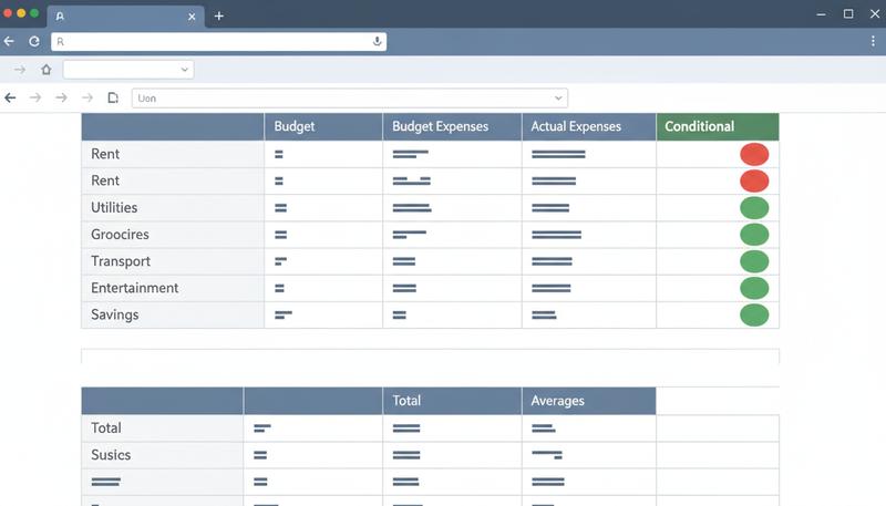
Practical Walkthrough: Building a Simple Budget Tracker
Let's put everything together. We'll build a small personal monthly budget tracker from scratch, using SUM, AVERAGE, IF, and IFERROR in real combination.
Here's what we're building:
| Column A | Column B | Column C | Column D |
|---|---|---|---|
| Category | Budgeted | Actual | Status |
| Rent | $1,200 | $1,200 | — |
| Groceries | $400 | $463 | — |
| Transport | $150 | $122 | — |
| Dining Out | $200 | $287 | — |
| Utilities | $100 | $94 | — |
| Entertainment | $100 | $145 | — |
| Total | |||
| Average |
Row 1 is the header row. Data runs from rows 2–7. Row 8 holds totals; row 9 holds averages.
Step 1: Set up the Status column
In D2, write a formula that says "Over" if the actual amount exceeds the budgeted amount, and "OK" if not:
=IF(C2>B2, "Over", "OK")
Copy this formula from D2 down to D7. Each row now automatically labels itself.
Step 2: Calculate totals
In B8 (Total for Budgeted column):
=SUM(B2:B7)
In C8 (Total for Actual column):
=SUM(C2:C7)
And now — a nested approach for the status of the overall budget. In D8:
=IF(C8>B8, "Over Budget", "On Track")
This checks the totals against each other to give you the big picture.
Step 3: Calculate averages
In B9 (Average monthly budget per category):
=AVERAGE(B2:B7)
In C9 (Average actual spend per category):
=AVERAGE(C2:C7)
Step 4: Add error protection for calculated columns
As your tracker grows, you might add a column E that shows the percentage of budget spent for each category — a formula like =C2/B2. That formula divides by B2, so if you ever add a new row but haven't filled in the budgeted amount yet, you'll get a #DIV/0! error staring back at you.
This is exactly when IFERROR earns its keep. Wrap the formula like this:
=IFERROR(C2/B2, "—")
Now if B2 is blank or zero, the cell shows a clean dash instead of an error code. Once you fill in a budget amount, the percentage appears automatically.
Alternatively, if you want to keep the Status column (column D) robust against partially filled rows, you can use a logical blank-check instead of relying on error handling:
=IF(ISBLANK(B2), "", IF(C2>B2, "Over", "OK"))
Read this as: "If B2 is empty, show nothing. Otherwise, check if the actual spend exceeds the budget and label accordingly." This approach doesn't suppress an error — it prevents a nonsensical comparison from running in the first place. Both techniques have their place; understanding the difference makes you a more deliberate spreadsheet builder.
What you've just built is a real, functional budget tracker. It automatically flags categories where you've overspent. It calculates your total and average spending. It updates the moment you type a new number. This isn't a toy example — it's something you could actually use.
Putting It in Perspective
The functions in this section — SUM, AVERAGE, COUNT, COUNTA, MIN, MAX, IF, IFERROR — are genuinely foundational. According to common usage patterns tracked across millions of spreadsheets, SUM and IF consistently rank as the most-used functions in the world. You've now learned both.
What matters more than memorizing syntax, though, is understanding the underlying logic: a function takes inputs, does a defined operation, and returns an output. Every single function in Google Sheets — all 400-odd of them — follows that same pattern. The inputs and operations differ, but the structure never changes.
That mental model is what makes learning the next function easy. In the upcoming section, we'll meet VLOOKUP — which uses that same structure to do something that feels almost magical the first time you see it: look up information in one table and pull it into another.
Only visible to you
Sign in to take notes.